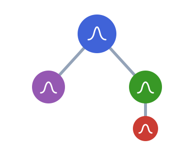
Time-, strata-, and covariate-varying distributions

A composed tree is stationary by default: every leaf is a fixed Distributions.jl distribution. Real delays are often non-stationary — an onset→admission delay shortens over a wave, a case-fatality ratio drifts, a delay differs by region. ComposedDistributions models this by generalising the leaf, not by adding a new composer verb: a leaf becomes a map from a context to a distribution, and instantiate resolves a whole tree against a context.

The design rationale (why non-stationarity lives here and not in the convolution layer, and how it relates to the uncertain-distributions work) is written up in design/0001-time-and-covariate-varying-distributions.md.

Two cases of one concept

Varying and Uncertain are the two deferred leaves: a leaf that is not yet a concrete distribution but a map to one. Varying maps an observed covariate (time, stratum) read from a Context and is resolved by instantiate; Uncertain maps a latent parameter draw (a value a sampler draws, with a prior) and is resolved by rand or collapsed by update. Both delegate silently to a fallback until resolved and share one resolution walk. Only the index differs — observed vs latent — so a leaf can be both, as the latent-parameters section below shows.

The three pieces

• Varying — a leaf holding a map covariate ↦ Distribution, the covariate it reads (default :time), and a reference distribution it behaves as when no context is supplied.

• Context — an open bag of covariates (Context(time = 5.0), Context(region = :north)).

• instantiate(tree, ctx) — resolves every varying leaf against the context and returns the same tree made concrete. It is the identity on fixed leaves and on a nothing context, so existing stationary trees are untouched.

Always instantiate before scoring or sampling

A Varying leaf behaves as its reference distribution (e.g. the t = 0 delay) until you call instantiate. Scoring or sampling a raw tree that still holds a Varying leaf — logpdf(tree, x), rand(tree) — does not error; it silently uses the reference, which is a wrong answer against real per-record times. Always resolve first (resolved = instantiate(tree, Context(time = t))) and score the resolved tree. In a fitting loop, guard the call with has_varying: @assert !has_varying(resolved).

A time-varying delay

using ComposedDistributions, Distributions

# An onset→admission delay whose scale grows with calendar time.
d = varying(t -> Gamma(2.0, 1.0 + 0.02t))

mean(d)                                    # the reference (t = 0)

2.0

mean(instantiate(d, Context(time = 10.0))) # the delay at t = 10

2.4

A Varying leaf drops into any composer as an ordinary leaf, because it is a UnivariateDistribution:

chain = sequential(:onset_admit => varying(t -> Gamma(2.0, 1.0 + 0.02t)),
    :admit_death => LogNormal(0.5, 0.4))

instantiate(chain, Context(time = 10.0))   # a concrete, stationary chain

Sequential (2 steps)
├─ onset_admit: Distributions.Gamma{Float64}(α=2.0, θ=1.2)
└─ admit_death: Distributions.LogNormal{Float64}(μ=0.5, σ=0.4)

Strata (a categorical covariate)

Time is just one covariate; a stratum is another. Name the covariate and pass a reference (there is no meaningful f(0.0) for a categorical index):

by_region = varying(r -> r === :north ? Gamma(2.0, 1.0) : Gamma(3.0, 1.5);
    covariate = :region, reference = Gamma(2.0, 1.0))

instantiate(by_region, Context(region = :south))

Distributions.Gamma{Float64}(α=3.0, θ=1.5)

Node-level variation (a time-varying CFR)

Because a Resolve is itself univariate, a whole node can vary — e.g. a case-fatality ratio that rises over time — with no new machinery:

cfr(t) = 0.2 + 0.02t
node = varying(t -> resolve(:death => (Gamma(1.5, 1.0), cfr(t)),
    :disch => Gamma(2.0, 1.5)))

instantiate(node, Context(time = 10.0))    # a concrete Resolve, CFR = 0.4

Resolve (2 outcomes)
├─ death (p = 0.4): Distributions.Gamma{Float64}(α=1.5, θ=1.0)
└─ disch (p = 0.6): Distributions.Gamma{Float64}(α=2.0, θ=1.5)

Choose resolves the same way

A Choose already selects an alternative by an observed data field. That is the categorical case of covariate indexing, so it resolves the same way: give the selector in the context and instantiate collapses to the chosen branch.

disj = choose(:index => Gamma(2.0, 1.0), :sourced => Gamma(4.0, 1.5))

instantiate(disj, Context(kind = :index))

Distributions.Gamma{Float64}(α=2.0, θ=1.0)

Latent parameters (the uncertain-distributions bridge)

An observed covariate (time, region) and a latent parameter (one a sampler draws) are the same covariate channel — only who fills the slot differs. A leaf keyed on a parameter name resolves against a context carrying that value, which with_covariates threads in alongside the observed covariates:

latent = varying(θ -> Gamma(θ, 1.0); covariate = :inc_shape,
    reference = Gamma(2.0, 1.0))

ctx = with_covariates(Context(time = 4.0); inc_shape = 2.5)  # sampler adds θ
instantiate(latent, ctx)

Distributions.Gamma{Float64}(α=2.5, θ=1.0)

This is the same generalisation as uncertain, along a different index. A Varying leaf keyed on a sampled parameter, resolved once the sampler fills the slot, is the bare bridge; Uncertain is the richer latent leaf that also carries each parameter's prior (so params_table rides it on the prior column and the estimation layer reads it), draws the marginal with rand, and collapses via update. Both are deferred leaves resolved by one machinery; a leaf keyed on an observed covariate whose per-level parameter is itself uncertain is both cases at once.

Feeding a recurrent / renewal operator

A recurrent (renewal) operator sweeps a delay kernel across a time series, one step per index — its "time" is the length of that vector. That operator is a consumer of the composed stack, not a composer itself; instantiate gives it exactly what it needs, a kernel per time step:

# Resolve the chain at each t, then collapse to its convolution kernel.
kernel_at(t) = observed_distribution(instantiate(chain, Context(time = t)))

kernels = [kernel_at(t) for t in 0:4]
mean.(kernels)                             # the kernel mean drifts with time

5-element Vector{Float64}:
 3.7860384307500734
 3.8260384307500734
 3.8660384307500735
 3.9060384307500735
 3.9460384307500735

Each kernel_at(t) is an ordinary Convolved distribution (a stationary kernel); non-stationarity is resolved before convolution, so a ConvolvedDistributions-based renewal step convolves it exactly as it would a fixed kernel. In other words: ComposedDistributions answers "what is the kernel at time t?", and the recurrent/renewal layer answers "apply it across the time axis." The recurrent operator itself is not part of this package — it lives in the renewal/time-series layer and calls kernel_at (as above) per step.

Learning more

• The full interface: Varying, varying, Context, with_covariates, instantiate in the Public API.

• The design rationale and open questions: design/0001-time-and-covariate-varying-distributions.md.